|
|
Home > Chapters > 3 >
1. Examples of global and local alignments of two proteins
Figures S3.1 and S3.2 present examples of global and local alignments of two proteins.
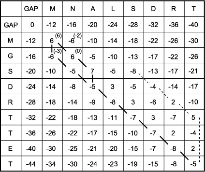
Figure S3.1. Global alignment of two protein sequences by the Needleman-Wunsch algorithm with enhancements by Smith and Waterman. This example illustrates a global alignment of two hypothetical sequences, sequence 1 = MNALSDRT and sequence 2 = MGSDRTTET. Notice the subsequence SDRT in the two sequences which one might expect to be aligned if the sequences are aligned properly.
|
A. Prepare a 10 x 11 matrix and place sequence 1 across the top of the matrix and sequence 2 down the left side. Leave an extra row and an extra column before each sequence labeled GAP to allow for gaps at the end of alignment. Fill in the extra row and column with the penalties for gaps of length zero to 8. The gap penalty used here is GAP = - 12- 4 (x - 1), where x is the length of the gap. -12 is the penalty for opening the gap in the alignment, and -4 is the penalty for each additional sequence character in the gap. The reason for choosing this particular penalty scheme is discussed below.
B. Fill in the score for each amino acid pair in the matrix. Shown in parentheses are examples for the four possible matches between the first two amino acids. These scores are taken from the log odds form of the Dayhoff scoring matrix at 250 PAMs described in Chapter 3.
C. Calculate the score in each of the above positions. The maximum score of the M/M position is the GAP/GAP score of 0 plus 6 for an M/M match, or 6. The arrow indicates the previous matrix position that was used to obtain a score of 6; i.e., the box labeled with a score of 0. Similarly, the maximum possible score in the N/M position is 6 - 12 (one gap penalty) = -6, that of the M/G position is 6 - 12 = -6, and that of the N/G position is 6 + 0 = 6 (no gap penalty). Note that each sequential row and column must be completed before moving to a lower row or more rightward column.
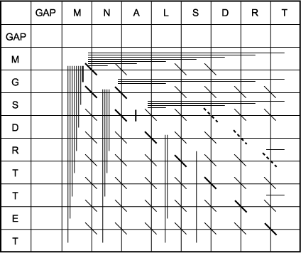
D. Complete the matrix by choosing at each position the maximum possible score (E). Keep track of all moves made to reach a maximum score at each position in a second matrix, the trace-back matrix (F).
 E. The scoring matrix is completed to find the highest score at each matrix position. The process started in C has been continued to fill in the entire matrix with the maximum possible score at each matrix position. The right column and lowest row are then examined for the highest possible score because the alignment is a global one, meaning that the alignment will end only when the end of one of the sequences has been reached. Any remaining unmatched sequence will be opposite gaps. The highest-scoring box in the right-hand column and lowest row is a 5 in row 7. If end gaps were not being penalized, this would be the end of the search for the best score. However, if the alignment were to end here, there are three unmatched positions left in sequence 2, and each will be opposite a gap. Thus, an additional penalty score for three gaps ( -20) corresponding to the heavy dotted line will have to be subtracted from 5, leaving an alignment score of 5 - 20 = -15. By subtracting any remaining end gap penalties from all positions in the last column and bottom row (not shown), one finds that the best score is actually -5 in the right-hand, lowest corner of the matrix obtained by a diagonal move to this position, giving a score of -8+3 = -5.
 F. The trace-back matrix is used to find which characters align. This matrix shows all of the moves made by the algorithm from one matrix position to another to calculate the maximum score at each position. Because the highest-scoring position in the last row and column is the -5 in the rightmost, lower corner, this position is in the alignment. Thus, the last T in each sequence will be matched. The task is to find a path back through the matrix using the moves made to get to that highest-scoring position and stopping at the beginning of one of the sequences. When the path turns from a previous diagonal move, a gap is placed opposite the next character in sequence 2 if the path turns upward and sequence 1 if it turns to the left. Two paths, shown as darker lines, are possible. These are also shown in part I above and correspond to the alignments 1 and 2 shown below. Note that if end gap penalties were not used, the path shown by the light dotted line in part I would be the correct alignment. This alignment, alignment 3, is also shown below. Note that wherever there are two paths leading to a matrix position, i.e., two possible ways of achieving that score, two alternative alignments will branch from that position. It is not too difficult to see that there are many possible paths through the scoring matrix that represent different alignments.
|
|
sequence 1   M  -  N  A  L  S  D  R  T
sequence 2   M  G  S  D  R  T  T  E  T
score        6 -12 1  0 -3  1  0 -1  3  =  -5
Alignment 1. Although this alignment has a low and insignificant score of -5, it is the best-scoring alignment that can be made between these two short sequences with the Needleman-Wunsch algorithm with end gaps penalized. Note that the score of -5 is also found at the lowest position in the last column, corresponding to the alignment of the last characters in the sequences. Normally, it only makes sense to use a global alignment method for producing an alignment between sequences that are about the same length and that are expected to align along their entire lengths. The end gap penalty forces the ends to align. For sequences that are quite similar along their lengths, using end gap penalties will not have the dramatic effect that it does in this hypothetical example.
|
sequence 1   M  N  -  A  L  S  D  R  T
sequence 2   M  G  S  D  R  T  T  E  T
score        6 -12 1  0 -3  1  0 -1  3  =  -5
Alignment 2. This second alignment is found by the trace-back procedure because there were two possible paths at one location in the matrix. This alignment scores slightly lower than the alignment 1 above. The difference is in the placement of a single gap opposite either a G or an S, and in the slightly higher score for the N/S versus the N/G alignment (1 vs. 0). This result illustrates that the dynamic programming alignment method may find more than one alignment having the same or almost the same score. Programs such as GCG GAP and BESTFIT can be set to provide several of these alternative alignments.
|
sequence 1   M  N  A  L  S  D  R  T  -  -  -
sequence 2   -  -  M  G  S  D  R  T  T  E  T
score        0  0 -1 -4  2  4  6  3  0  0  0  =  10
Alignment 3. (no end gap penalty included). On initial observation, this alignment has a great deal more appeal than the above two and has a much higher score. However, all of the gaps needed to make the alignment have been put on the ends, where they do not count. Leaving out end gaps also makes the analysis less rigorous mathematically (they appear in the rigorous proofs) and leaves doubt as to whether or not evolutionary conclusions may be drawn (Smith and Waterman 1981a,b). There is a positive effect of helping to identify the region of similarity SDRT without scoring end gaps, but using the Needleman-Wunsch algorithm, this region could still be missed if this amino acid pattern was broken by higher-scoring neighboring alignments. The Smith-Waterman local alignment algorithm discussed below is specifically designed to find such conserved patterns of local alignment.
|
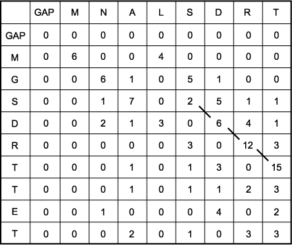
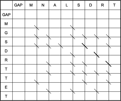
Figure S3.2. Local sequence alignment by the Smith-Waterman algorithm.
 A. Scoring matrix for Smith-Waterman alignment of sequence 1, MNALSDRT, and sequence 2, MGSDRTTET. These same sequences, the PAM250 scoring matrix and gap penalty scores (-12 and -4 for gap opening and gap extension penalties, respectively) for internal and end gaps, were used. The major difference between this scoring matrix and the Needleman-Wunsch matrix is that there are no negative scores in the Smith-Waterman scoring matrix. The effect of this change is that an alignment can begin anywhere without receiving a negative penalty from a previously low- scoring alignment. Once an alignment has been built, it stops when negative alignment scores or the introduction of gaps reduces the following alignment scores to 0. Thus, only a portion of each sequence that was in this high- scoring region will be reported. Note that in this example the initial end gap penalty does not have any effect because all first row and column scores are 0, the minimum allowed by the Smith-Waterman algorithm. Because a gap penalty at the end of the alignment produces a score of zero, the end gap penalty similarly has no effect.
 B. The trace-back matrix of the above Smith-Waterman scoring matrix. To find the optimal local alignment, the highest-scoring position in the scoring matrix is located (15), and the trace-back from this position is followed up to a zero in the matrix. The resulting sequence alignment is shown below. As opposed to the complex moves in the Needleman-Wunsch matrix, which are designed to test many combinations of matches, mismatches, and gaps, only simple diagonal moves were made in the Smith-Waterman matrix. Thus, there is only one alignment starting from the highest position. However, many other lower-scoring alignments are apparent, such as the second highest-scoring alignment of MNA with MGS starting at the position that scores 7. Note that this second alignment does not include any of the same amino acids, and not even any of the same aligned amino acids, that were used in the first alignment. It is possible to have multiple local alignments that do use the same aligned amino acid pairs, as there was in the global alignment example given above, but there are no examples in this matrix. The distinctions regarding which alignments use the same aligned pairs, which use the same residues in a different alignment, and which use entirely different residues are described in Chapter 3.
sequence 1    S D R T
sequence 2    S D R T
score         2 4 6 3 = 15
|
C. Sequence alignment determined by the above procedure. Note that the score of the alignment is the same as that shown by the highest-scoring position in the scoring matrix. The inclusion of any additional sequence would reduce the score below 15.
|
|
|
|
| © 2004 by Cold Spring Harbor Laboratory Press. All rights reserved. |
 |
| No part of these pages, either text or image, may be used for any purpose other than personal use. Therefore, reproduction, modification, storage in a retrieval system, or retransmission, in any form or by any means, electronic, mechanical, or otherwise, for reasons other than personal use, is strictly prohibited without prior written permission. |
|
|
|